Blog

Hello! And welcome to today’s post! I’m going to discuss a bit on functional equations, and several methods for solving them. At the end, I list a few great textbooks if you want to learn more.

A functional equation is a relation involving a function and different variable arguments. Functional equations may involve no explicit variable expression, or they may contain an explicit expression of the independent variable(s). Cauchy’s equations furnish classic examples of the first case:

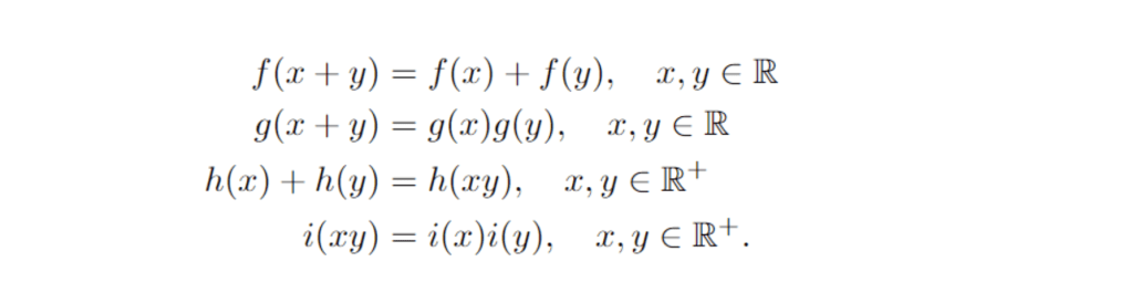
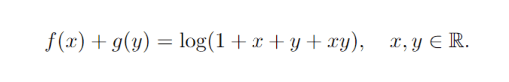
An example with some explicit variable expression is

The study of functional equations is a vast field, which is particularly difficult because there is not a very straightforward theory for solutions. In contrast to the study of linear algebraic, difference, or differential equations, there is not a universal theory as to how many independent solutions we can expect from a nonlinear equation. Furthermore, a functional equation not involving derivatives imposes no requirement for smoothness of solutions. So, in principle there may be various non-smooth solutions.

For this post, I will simply illustrate how some functional equations can be solved by converting them to differential equations. This approach enables us to find smooth solutions to some equations. This is the first method I want to discuss, which will be employed on the first two of Cauchy’s equations.

As with any equation, the idea of “solving it” amounts to eliminating the non-trivial dependencies. In the case of differential equations, these are dependencies are derivatives. For functional equations, these are dependencies on complex arguments of independent variables. A functional equation is solved when we are able to extract a relationship with the argument “x” alone, and no nonlinear expressions involving f(x).

Let’s start with Cauchy’s first equation. The idea is to take partial derivatives as needed, in order to form a system of equations in which the terms involving non-trivial arguments can be eliminated.

Taking the partial derivative of the first equation with respect to x, and then with respect to y yields:

Subtracting the two equations tells us that

Because we have a function of x identically equal to a function of y, the two must equal a constant.

So, the solutions are simply the linear functions.

Let us continue with the second equation. Differentiating first wrt x, then wrt y, we find that

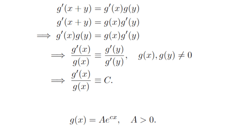
So, the solutions are exponential functions!

I will leave you as the reader to solve the third and fourth equations.

Here is a more complicated example, where the derivatives are not as easy. This is d’Alembert’s equation.

Taking the second partial derivative wrt x gives us

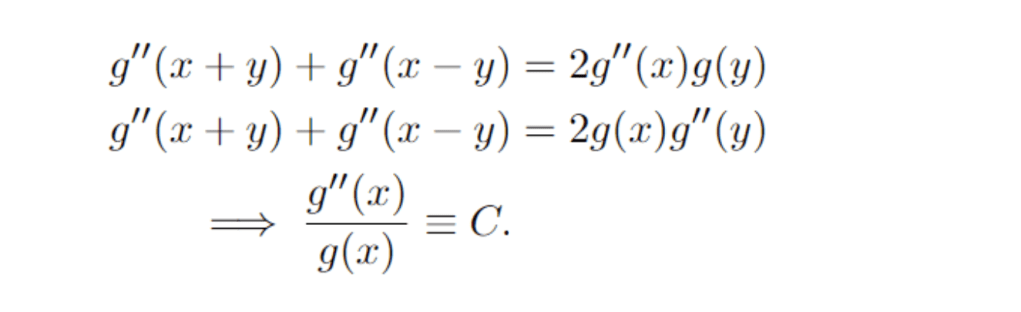
As you may recall from a class in differential equations, this equation has very different solutions depending on the value of C. If C<0, we get sinusoidal solutions, and if C>0, we get exponential solutions. Finally, if C = 0, the solutions are linear functions.

Because we want the solution to vanish at infinity, zero is the only valid solution.

As an exercise, try to solve the equation below, finding all valid f,g such that

In this post, I will discuss an interesting integration technique not commonly taught in school. We will review integration by parts first, and then discuss a technique called complexification of the integral. Both methods are useful for integrating trigonometric functions. For today’s application, I will show how complexification can uncover interesting properties of integrals used in Fourier analysis.

A common integral for first learning integration by parts is one involving an exponential – cosine product. Because the cosine function repeats itself after two derivatives (or integrations), we need to apply integration by parts twice to solve the problem. Here is the process.

Students will typically find this example challenging because they want the integration by parts to directly lead to the solution. But here, due to the periodicity of cosine, we can only find a result involving the original integral. We thus need to solve the equation by moving the integral of interest to one side.

You might be wondering if there is a direct way to compute an integral like this — an there is! Enter complexification.

The idea is to express trig functions in terms of the complex exponential, which is credited to Euler and known as Euler’s formula.

By introducing (-x), and knowing that cosine is an even function, and sine an odd function, we can derive formulas for sine and cosine.

We can substitute these formulas in for sine and cosine, and then apply the integration rule for the exponential function. For our problem above, which involves only cosine, it is arguably easier to just take the real part of the integral. Real and imaginary parts may be denoted as follows.

Now, the above problem may be solved as follows.

Of course, we find the same result as with integration by parts. For e^x sin(x), you would follow the same process, but instead taking the imaginary part.

Now, in computing Fourier series for functions, there are various useful formulas involving products of sines and cosines with different frequencies, which might be introduced in a course on partial differential equations. A great webpage for these formulas is on Paul’s Math Notes.

Because sine and cosine are odd and even, respectively, it should be clear that integrating any product of these functions over a full period will yield zero as the result. What is not so obvious (at least to me) is why the integrals of products of two cosine functions or two sine function with different frequencies over a full period are also zero. The specific result I will show in the remainder of this post is

Here, m and n are integers. For simplicity, I will take L = 1. The following calculation is somewhat tedious, but every mathematician should see it at least once 😉

As an exercise, you can practice this calculation with the product of sines with m not equal to n. This integral will also be zero.

I hope you enjoyed this post and found it helpful. If so, please give me a like, and comment if you have a particular topic you are interested in. I also welcome other math bloggers, if you want me to check out your website.

When first learning integration rules in calculus, we start with the power rule. The differentiation and integration of power functions is very simple and can be automated in computation software.

The integration formula follows directly from the rule for the derivative. If we differentiate the second formula, we get the integrand.

You might have learned a couple ways for proving this formula. One is to directly apply the definition of the derivative, making use of the binomial formula and the limit techniques. An easier way, for integral powers excluding -1, is to simply use induction on n. We know that the derivative of x is 1 from the definition.

Now, we assume that for some positive integer n greater than or equal to 1,

and show that the formula holds for n+1. For this, we use the product rule.

Now, for negative integral powers (excluding -1), we just use the formula with the quotient rule.

Of course, polynomials become a straight-forward matter, since the derivative and integral are linear — we can distribute the operators through a linear combination of the monomials of degrees less than or equal to n, for a polynomial of degree n.

Now comes the main point of this post. We want to understand the case for -1. As is customary in mathematics, when we don’t know what a function is, we “invent” the function using an integral definition. Let the integral of 1/x be denoted by L(x).

It should be clear as to why c > 0. We cannot integrate over the singularity at 0 (the integral would become infinite). We can say several things about this function right away. First of all, the function is zero when c = 1 and x = 1. Secondly, the integral is positive for x > c, and negative for x < c. Now, suppose a and b are both positive numbers. Then, using fundamental integration properties (u-substitution, which is essentially the chain rule in reverse) and linearity, and choosing c = 1 we find that:

Now, because L(1) = 0, we can also show a formula for a/b.

Is is now clear that this function, which is continuous and satisfies the above properties, must be the natural logarithm!

This, in my opinion, would be a great exercise for calc 1 students. Deriving the rules of the natural log from the integral definition.

If you enjoyed reading this post, please leave me a comment :).